Distributed Deep Learninig - Part 1

Note: Meanwhile I published my Master Thesis on parallelizing gradient descent which provides a full and more detailed description of the concepts described below.

In the following blog posts we study the topic of Distributed Deep Learning, or rather, how to parallelize gradient descent using data parallel methods. We start by laying out the theory, while supplying you with some intuition into the techniques we applied. At the end of this blog post, we conduct some experiments to evaluate how different optimization schemes perform in identical situations. We also introduce dist-keras, which is our distributed deep learning framework built on top of Apache Spark and Keras. For this, we provide several notebooks and examples. This framework is mainly used to test our distributed optimization schemes, however, it also has several practical applications at CERN, not only because of the distributed learning, but also for model serving purposes. For example, we provide several examples which show you how to integrate this framework with Spark Streaming and Apache Kafka. Finally, these series will contain parts of my master-thesis research. As a result, they will mainly show my research progress. However, some might find some of the approaches I present here useful to apply in their own work.

Introduction

Unsupervised feature learning and deep learning has shown that being able to train large models on vasts amount of data can drastically improve model performance. However, consider the problem of training a deep network with millions, or even billions of parameters. How do we achieve this without waiting for days, or even multiple weeks? Dean et al. [2] propose a different training paradigm which allows us to train and serve a model on multiple physical machines. The authors propose two novel methodologies to accomplish this, namely, model parallelism and data parallelism. In the following blog post, we briefly mention model parallelism since we will mainly focus on data parallel approaches.

Sidenote: In order to simplify the figures, and make them more intuitive, we negate the gradient $\nabla f$ without adding a $-$ sign in front. Thus, all gradient symbols in the following figures will be negated by default, unless stated otherwise. I actually forgot to negate the gradients in the figures, so mentioning this is rather an easy fix. However, this will be corrected in the final version of the master thesis.

Model parallelism

In model parallelism, a single model is distributed over multiple machines. The performance benefits of distributing a deep network across multiple machines mainly depends on the structure of the model. Models with a large number of parameters typically benefit from access to more CPU cores and memory, thus, parallelizing a large model produces a significant performance increase, and thereby reducing the training time.

Let us start with a simple example in order to illustrate this concept more clearly. Imagine having a perceptron, as depicted in Figure 1. In order to parallelize this efficiently, we can view a neural network as a dependency graph, where the goal is to minimize the number of synchronization mechanisms, assuming we have unlimited resources. Furthermore, a synchronization mechanism is only required when a node has more than 1 variable dependency. A variable dependency is a dependency which can change in time. For example, a bias would be a static dependency, because the value of a bias remains constant over time. In the case for the perceptron shown in Figure 1, the parallelization is quite straightforward. The only synchronization mechanism which should be implemented resides in output neuron since $y \triangleq \sigma(\sum_i w_ix_i)$ where $\sigma$ is the activation function of the output neuron.

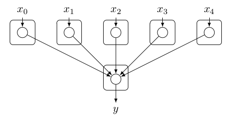
Figure 1: A perceptron partitioned using the model parallelism paradigm. In this approach every input node is responsible for accepting the input $x_i$ from some source, and multiplying the input with the associated weight $w_i$ . After the multiplication, the result is sent to the node which is responsible for computing $y$ . Of course, this node requires a synchronization mechanism to ensure that the result is consistent. The synchronization mechanism does this by waiting for the results y depends on.

Data parallelism

Data parallelism is an inherently different methodology of optimizing parameters. The general idea is to reduce the training time by having $n$ workers optimizing a central model by processing $n$ different shards (partitions) of the dataset in parallel. In this setting we distribute $n$ model replicas over n processing nodes, i.e., every node (or process) holds one model replica. Then, the workers train their local replica using the assigned data shard. However, it is possible to coordinate the workers in such a way that, together, they will optimize a single objective. There are several approaches to achieve this, and these will be discussed in greater detail in the coming sections and blog posts.

Nevertheless, a popular approach to optimize this objective is to employ a centralized parameter server. A parameter server is responsible for the aggregation of model updates, and parameter requests coming from different workers. The distributed learning process starts by partitioning a dataset into $n$ shards. Every individual shard will be assigned to a particular worker. Next, a worker will sample mini-batches from its shard in order to train the local model replica. After every mini-batch (or multiple mini-batches), the workers will communicate a variable with the parameter server. This variable is in most implementations the gradient $\nabla f_i(x)$ . Finally, the parameter server will integrate this variable by applying a specific update procedure which knows how to handle this variable. This process repeats itself until all workers have sampled all mini-batches from their shard. This high-level description is summarized in Figure 2.

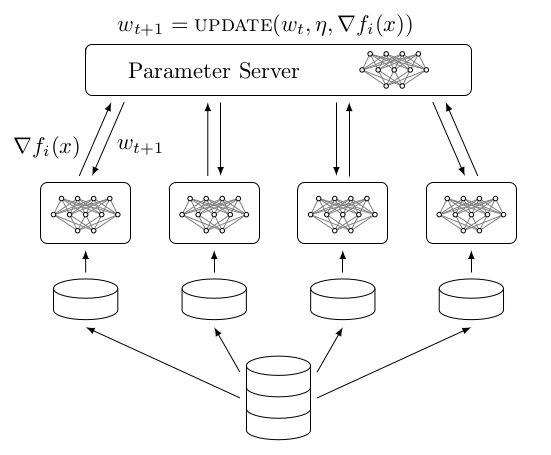
Figure 2: Schematic representation of a data parallel approach. In this methodology we spawn $n$ workers (not necessarily on different machines), and assign a data shard (partition) of the dataset to every worker. Using this data shard, a worker $i$ will iterate through all mini-batches to produce a gradient, $\nabla f_i(x)$ for every mini-batch $x$ . Next, $\nabla f_i(x)$ is send to the parameter server, which will incorperate the gradient using an update mechanism.

Approaches

In this section we discuss several approaches towards parallelizing gradient descent (GD). This is not an intuitive task since gradient descent is an inherently sequential algorithm where every data point (instance) provides a direction to a minimum. However, training a model with a lot of parameters while using a very large dataset, will result in a high training time. If one would like the reduce the training time, the obvious choice would be to buy better, or rather, more suitable hardware (e.g., a GPU). However, this is not always possible. For this reason, several attempts have been made to parallelize gradient descent. In the following subsections, we will examine some of the popular approaches to parallelize gradient descent, and provide some intuition into these techniques work, and how they should be used.

Synchronous Data Parallel Methods

There are two distinct approaches towards solving data parallelism. Personally, the most conceptually straightforward one is synchronous data parallelism. In synchronous data parallelism, as depicted in Figure 3, all workers compute their gradients based on the same center variable. This means whenever a worker is done computing a gradient for the current batch, it will commit a parameter (i.e., the gradient or the parameterization of the model) to the parameter server. However, before incorporating this information into the center variable, the parameter server stores all the information until all workers have committed their work. After this, the parameter server will apply a specific update mechanism (depending on the algorithm) to incorporate the commits into the parameter server. In essence, one can see synchronous data parallelism as a way to parallelize the computation of a mini-batch.

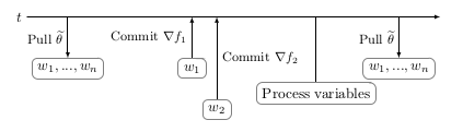
Figure 3: In a synchronous data parallel setting, one has $n$ workers (not necessarily on different machines). At the start of the training procedure, every worker fetches the most recent center variable. Next, every worker will start their training procedure. After the computation of the gradient, a worker commits the computed information (gradient or parametrization, depending on the algorithm) to the parameter server. However, due to unmodeled system behaviour, some workers might induce a significant delay, which results in other workers to be taskless while still consuming the same memory resources.

However, due to unmodeled system behaviour of the workers, workers might commit their results with a certain delay. Depending on the system load, this delay can be quite significant. As a result, this data parallel method is a case of the age-old saying "a synchronous data parallel method is only as strong, as the weakest worker in the cluster" :-).

Model Averaging

In essence, this is a data parallel approach as mentioned in the introduction. However, in contrary to more conventional data parallel approaches, there is no parameter server. In model averaging, every worker will get a copy of the model at the start of the training period. However, one can have different weight initialization techniques for the workers to cover more of the parameter space after several iterations, as shown in Figure 4. Though, it is not recommended to do this since this will result in very different solutions for every worker. Thus wasting initial iterations converging to a "good solution" on which all workers "agree". However, this problem is related to most distributed optimization algorithms discussed here, and will be discussed in more detail in the following blog posts.

After every worker is initialized with a copy of the model, all workers start the training procedure independently from each other. This means that during the training procedure, no communication between the workers occurs. Thus, eliminating the communication overhead that is present in approaches with parameter servers. After the end of an epoch, i.e., a full iteration of the dataset, the models are aggregated and averaged on a single worker. The resulting averaged model will then be distributed to all workers, where the training process repeats until the averaged model converges.

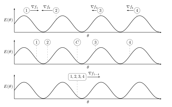
Figure 4: In this setting we have 4 independent workers, each having a randomly initialized model. In order to simplify the situation, let us assume we can obtain the gradient directly from $E(\theta)$ , which is our loss function. In model averaging, every worker only applies gradient descent to its own model without communicating with other workers. After the end of an epoch, as shown in the center plot, the models are averaged in order to produce a central model. In the following epoch, the central model will be used as a starting point for all workers.

EASGD

EASGD, or Elastic Averaging SGD, introduced by Zhang et al. [3], is a distributed optimization scheme designed to reduce communication overhead with the parameter server. This is in contrast to approaches such as DOWNPOUR, which most of the time require a small communication window in order to converge properly. The issue with a small communication window is that the learning process needs to be stopped in order to synchronize the model with the parameter server, and as a result, limiting the throughput of the training process. Of course, the number of parameters in a model is also an important factor. For example, one can imagine that having a model with 100 MB worth of parameters could severely influence the training performance if every 5 mini-batches a synchronization with the parameter server would occur. Furthermore, the authors state that due to the distributed nature, exploration of the nearby parameter space by the workers actually improves the statistical performance of a model with respect to sequential gradient descent. However, at the moment, we do not have any evidence to support this claim, nor to deny it. What we do observe, is that the statistical performance of a model after a single epoch, is usually (significantly) less than a single epoch of Adam (sequential training) and ADAG (distributed training). However, if we would let EASGD reach the same amount of wallclock training time, then we still have an identical or slightly worse model performance. So there is evidence to suggest that this claim is not completely true, at least, in the case of EASGD. This however, requires more investigation.

The authors solve the communication constraint by applying an "elastic force" between the parameters of the workers and the center variable. Furthermore, due to the elasticity and reduction in communication with the parameter server, the workers are allowed to explore the surrounding parameter space. As stated above, the authors claim that allowing for more exploration can be beneficial for the statistical performance of the model. However, we argue that, as in model averaging, this will only work well if the workers are in the neighbourhood of the center variable, we will show this empirically in the Experiments section. However, in contrast to model averaging, the workers are not synchronized with the center variable. This begs the question, how does EASGD ensure that the workers remain in the "neighbourhood" of the center variable? Because as in model averaging, too much exploration of the parameter space actually deteriorates the performance of the center variable, and may prevent convergence, because the workers cover inherently different spaces of the parameter space, as shown in Figure 4. However, if the elasticity parameter is too high, exploration will not take place at all.

\theta^i_{t+1} = \theta^i_t - \eta\nabla f(\theta^i_t) - \eta\rho(\theta^i_t - \theta^c_t)

(1)

\theta^c_{t+1} = (1 - n\eta\rho) \theta^c_t + \eta\rho(\frac{1}{n} \sum_{i = 0}^{n} \theta^i_t)

(2)

To fully understand the implications of the EASGD equations, as shown in Equation 1 and Equation 2, we refer the reader to Figure 5, which shows the intuition behind the elastic force. Having two vectors, the gradient $\nabla f$ , and the elastic difference $\eta\rho(\theta^i_t - \theta^c_t)$ where $\eta$ is the learning rate and $\rho$ is the elasticity parameter, the authors say when $\rho$ is small, you allow for more exploration of the parameter space. This can be observed from Figure 5. When $\rho$ is small, the vector $\eta\rho(\theta^i_t - \theta^c_t)$ will be small as well (unless the distance between the worker and the center variable is large). As a result, the attraction between the center variable and the worker is small, thus, allowing for more exploration of the parameter space.

Analogously, imagine that you are walking with your dog, and the dog is responsible for getting you home (guiding you to a minimum). If you would let your dog drift too far away from you (because you have a leash which is very flexible (small $\rho$ )). In the most extreme case, the dog will get home without you because your leash was simply too flexible. As a result, the dog could not pull you home. At this point you think, maybe I should buy more dogs? Thinking that together they will help you. However, due to the nature of these creatures you soon realize that instead of going home, they all go to different places (multiple workers in the parameter space having different inputs, e.g., one dog sees a particular tree, while an other dog sees a bush, etc.). From this experience, you notice that the problem is the leash, it is way too flexible because the dogs are all over the place. As a result, you buy a less flexible leash, with the effect that the dogs stay closer to you, and eventually "pull" together to bring you home faster.

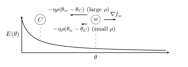
Figure 5: The worker variable $w$ is exploring the parameter space in order to optimize $C$ . However, the amount of exploration is proportional by the elasticity factor $\rho$ , and the difference $(\theta^w_t - \theta^C_t)$ . In general, when $\rho$ is small, you allow for more exploration to occur. It is to be noted, that as in model averaging, too much exploration will actually deteriorate the statistical performance of a model (as shown in the first subfigure of Figure 4), because the workers do not agree on a good solution. Especially when you take into account that the center variable is updated using an average of the worker variables, shown in Equation 2.

Now, from Equation 1 and the intuition above, we can expect that for some worker update $i$ within a communication window, the accumulated gradient is larger or equal to the elastic force. As a result, this prevents the workers from further exploration (as expected). However, a significant side-effect is that the following gradient computations are wasted since they are countered by the elastic difference, as shown in Figure 5. Using the analogy from above, this is equivalent to a situation where no matter how hard a dog is trying to pull, you just don't let it go any further. Thus, the efforts of the dog are wasted. This condition is described by Equation 3.

- \sum_i - \eta\nabla f(x_{t + i};\theta_{t + i}) \geq -\eta\rho(\theta_{t + i + 1} - \theta_t^C)

(3)

A straightforward technique to prevent the squandering of computations after the condition described by Equation 3, is to simply check for this condition after the computation of every mini-batch. When this condition is met, then the term $\sum_i - \eta\nabla f(x_{t + i};\theta_{t + i})$ is communicated with the parameter server. As a result, we do not waste any computations, and furthermore, we loose a hyperparameter since the communication window is now controlled (indirectly) by the hyperparameter $\rho$ , which controls the elastic force. In essence, the core idea of ADAG (which will be mentioned later in this blog post), can also be applied to this scheme to even further improve the quality of the gradient updates, and making the optimization scheme less sensitive to other hyperparameters, e.g., the number of parallel workers.

Asynchronous Data Parallel Methods

In order to overcome the significant delays induced by loaded workers in synchronous data parallelism, and thereby decrease the training time even further, let us simply remove the synchronization constraint. However, this imposes several other effects, and some of them are not very obvious. The conceptually simplest, is parameter staleness. Parameter staleness is simply the number of commits other workers performed between the last pull (center variable synchronization), and the last commit (parameter update) of the current worker. Intuitively, this implies that a worker is updating a "newer" model using gradients based on a previous parametrization of that model. This is shown in Figure 6.

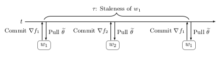
Figure 6: In asynchronous data parallelism, training time is even further reduced (on average) due to the removal of the synchronization mechanism in synchronous data parallelism. However, this induces several effects such as parameter staleness, and asynchrony induced momentum.

Note: It is not required to read the paragraphs below, unless you really want to. However, the take-away point is: increasing the number of parallel workers behaves like adding more momentum.

The other, less intuitive side-effect is asynchrony induced momentum [1]. Roughly stated, this means that adding more workers to the problem also adds more implicit momentum to the optimization process. This implicit momentum is the result of the queuing model required by asynchrony. Note that some approaches, such as Hogwild! do not require locking mechanisms, since they assume sparse gradient updates. However, distributed SGD works with dense gradient updates as well. We also confirm the statements of the authors that adding more asynchronous workers to the problem actually deteriorates the statistical performance of the model when using algorithms which do not take staleness and asynchrony into account. Furthermore, they state that the behaviour of an asynchronous algorithm is roughly described by Equation 4. Which implies that the implicit momentum produced by asynchrony is $(1 - \frac{1}{n})$ .

E[\theta_{t+1} - \theta_t] = (1 - \frac{1}{n})E[\theta_t - \theta_{t-1}] - \frac{1}{n}\eta E \nabla f_i(\theta_t)

(4)

But personally, I think this is not the complete story. I agree with the nicely formalized queueing model, and that in general, an increase in the number of asynchronous workers decreases the statistical performance of a model (we also observe this in our experiments). However, I would say that the effect rather behaves like momentum, but cannot be necessarily be defined as such (with ADAG, we do not observe this effect, at least for 30 parallel processes). We will go more in-depth into this topic in the following blog posts, since this is still a topic that requires some more research on my part.

Asynchronous EASGD

The update scheme of asynchronous EASGD is quite similar, however, there are some important details. In the following paragraphs we will call the vector $- \eta\rho(\theta^i_t - \theta^c_t)$ the elastic difference, and thereby following the notation of the paper. Remember that in the synchronous version this vector is actually used to enforce the exploration policy. Meaning, in Equation 1 this vector has the task to not let a worker drift too "far" from the center variable. Repeating the analogy with the dogs, imagine having a dog with an elastic leash. The further the dog walks away from you (the center variable), the stronger the force will be to pull it back. As a result, at some point the force the dogs exerts will be equal to the force the elastic leash exerts in the opposite direction. At this point, the dog cannot move any further. This is exactly what happens when the elastic difference is applied to a worker, as shown in Figure 5.

In the asynchronous version, the elastic difference has the same function. However, it will also be used to update the center variable. As stated in the paragraph above, the elastic difference is actually used to limit exploration. However, if we negate the elastic difference, which is $+ \eta\rho(\theta^i_t - \theta^c_t)$ , then the elastic difference can be used to optimize the center variable (reverse the arrow in Figure 5), while still holding true to the communication constraints EASGD is trying to solve.

DOWNPOUR

In DOWNPOUR, whenever a worker computes a gradient (or a sequence of gradients), the gradient is communicated with the parameter server. When the parameter server receives the gradient update from a worker, it will incorporate the update in the center variable, as shown in Figure 7. Contrary to EASGD, DOWNPOUR does not assume any communication constraints. Even more, if frequent communication with the parameter server does not take place (in order to reduce worker variance), DOWNPOUR will not converge (this is also related to the asynchrony induces momentum issue, see Figure 8). This is because of the same issues discussed in the sections above. If we allow the workers to explore "too much" of the parameter space, then the workers will not work together on finding a good solution for the center variable. Furthermore, DOWNPOUR does not have any intrinsic mechanisms in place to remain in the neighbourhood of the center variable. As a result, if you would increase the communication window, you would proportionally increase the length of the gradient which is sent to the parameter server, thus, the center variable is updated more aggressively in order to keep the variance of the workers in the parameter space "small".

Figure 7: Animation of DOWNPOUR with 20 parallel workers (blue) with identical learning rates which are trying to optimize a single objective (center variable, red) compared to regular sequential gradient descent (green). From this animation we can observe the momentum induced by the asynchrony of the parallel workers, as discussed above.

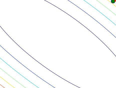
DOWNPOUR with too much implicit momentum

Figure 8: Animation of DOWNPOUR with 40 parallel workers. In this case, the implicit momentum produced by the number of workers causes the algorithm to diverge.

ADAG

We noticed that a large communication window is correlated with a decline in model performance. Using some simulations (like DOWNPOUR, as shown above), we noticed that this effect can be mitigated when you normalize the accumulated gradient with the communication window. This has several positive effects, for one, you are not normalizing with respect to the number of parallel workers, thus, as a result, you are not losing the (convergence speed) benefit of parallelizing gradient descent. This has as a side-effect, that the variance of the workers with respect to the center variable will also remain small, thus contributing positively to the central objective! Furthermore, because of the normalization, you are less sensitive to hyperparametrization, especially regarding the communication window. However, it is to say that a large communication window typically also degrades the performance of the model because you allow the workers to explore more of the parameter space using the samples from their data shard. In our first prototype, we adapted DOWNPOUR to fit this idea. We observed the following results. First, we observe a significant increase in model performance, even compared to a sequential optimization scheme such as Adam. Second, compared to DOWNPOUR, we can increase the communication window with a factor 3. Thus, allow to utilize the CPU resources more efficiently, and decreasing the total training time even further. Finally, normalizing the accumulated gradient allows us the increase the communication window. As a result, we are able to match the training time of EASGD, and achieve the roughly the same (sometimes better, sometimes worse).

\Large \frac{\sum_{i=0}^{\tau}-\eta\nabla f(x_{t + i};\theta_{t + i})}{\tau}

(5)

To conclude, the core idea of ADAG, or asynchronous distributed adaptive gradients, can be applied to any distributed optimization scheme. Using our observations, and intuition (especially with respect to implicit momentum due to asynchrony), we can make a calculated guess that the idea of normalized accumulated gradients can be applied to any distributed optimization scheme. However, we need to conduct several experiments in order to verify this claim. ADAG will be discussed in detail in the following blog posts.

Experiments

In the following experiments we set up the different optimization schemes against each other, i.e. (sequential) Adam, (distributed) DOWNPOUR, Asynchronous EASGD, and ADAG, and evaluate them using the MNIST dataset (samples are shown in Figure 10). We will use the following parameters during our experiments:

Multilayer perceptron with 1 000 000 trainable parameters (~4 MB model) (complete model summarized below)
4 sample mini-batches
1 epoch
Parallelism factor: 1
Adam as worker optimizer
Communication windows:
- DOWNPOUR: 5
- ADAG: 5
- Asynchronous EASGD: 32
20 parallel workers:
- 10 compute nodes with 10 Gbps network cards
- 2 processes per compute node (32 cores)

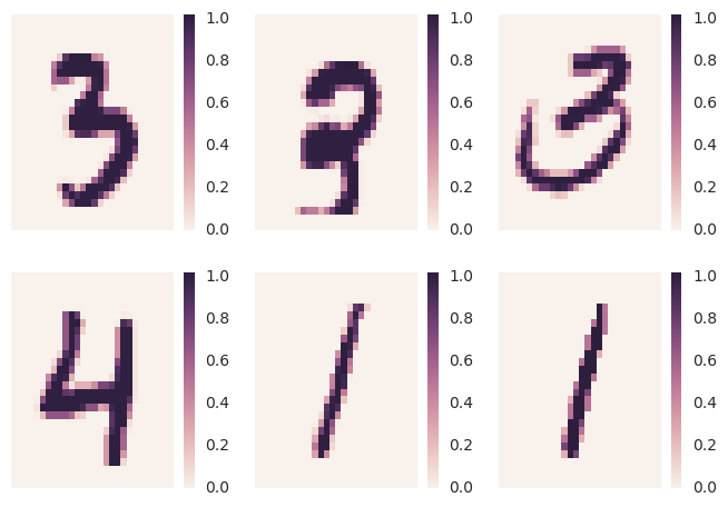
Figure 10: The MNIST dataset is a collection of handwritten digits. This dataset is usually used as a "unit test" for optimization algorithms. Every sample consists of 784 pixels, with values ranging between 0 and 255. We normalize these using our framework dist-keras, which is built on top of Apache Spark, thus, profiting from the parallelization.

In the following experiments we evaluate the accuracy of the central variable, and the training time (wallclock) compared to the number of parallel workers. Although this is a relatively small dataset, it gives us some indications into the scaling abilities of the optimization schems. In the following blog posts we will also focus on large scale deep learning, meaning, we will handle very large datasets and train models in a data parallel setting.

DOWNPOUR

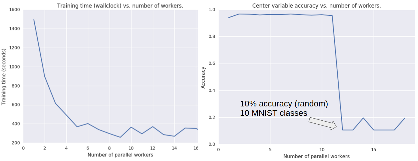
Figure 11: A key observation in this experiment is that DOWNPOUR actually diverges when it reaches a critical amount of implicit momentum, as shown in Figure 8. We made this observation in several other datasets as well. However, the constantly declining performance the authors in [1] is not observed. Rather, we have a sudden decline in model performance. This is rather contradictory to the claims made in [1]. According to their theory, we should not see a sudden decline in model performance, but rather a steady decline. As a result, we think that their statement "there exists a limit to asynchrony" is false as well. Though, their intuition is correct! Furthermore, on the left, we see the scaling of the algorithm. We actually expected that the scaling should work better, however, this could be because of the unbalanced partitions (we are doing experiments with other partitioners to correct for this) and relatively small dataset.

Asynchronous EASGD

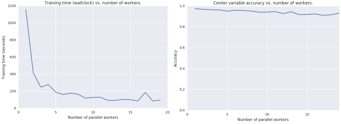
Figure 12: As stated above, EASGD is an algorithm designed with communication constraints in mind, which is a realistic constraint. As a result, the authors incorporate an elastic force which allows the worker to explore a certain area of the neighbouring parameter space w.r.t. the center variable. As a result, it will not have an immediate decline in model performance, as observed in DOWNPOUR, but rather a steady decline. This decline (with respect to the number of model performance), is due to the increased amount of staleness (since the center variable will have covered more distance because of the queuing model) compared to the worker. As a result, the positive information a worker can contribute is proportional to the elastic difference, and this elastic difference will be smaller when the number of parallel workers is higher (due to parameter staleness). However, since EASGD scales very well with the number of workers, we simply match the training time of ADAG or DOWNPOUR. However, even if we would match the training time, EASGD usually results in a lower accuracy compared to ADAG. This is phenomena is subject to further study, as it is not really completely understood why this is actually happening. Furthermore, it also consumes more CPU compared to ADAG, if we would match the model performance of ADAG (ADAG spends a lot of time waiting for network operations).

ADAG

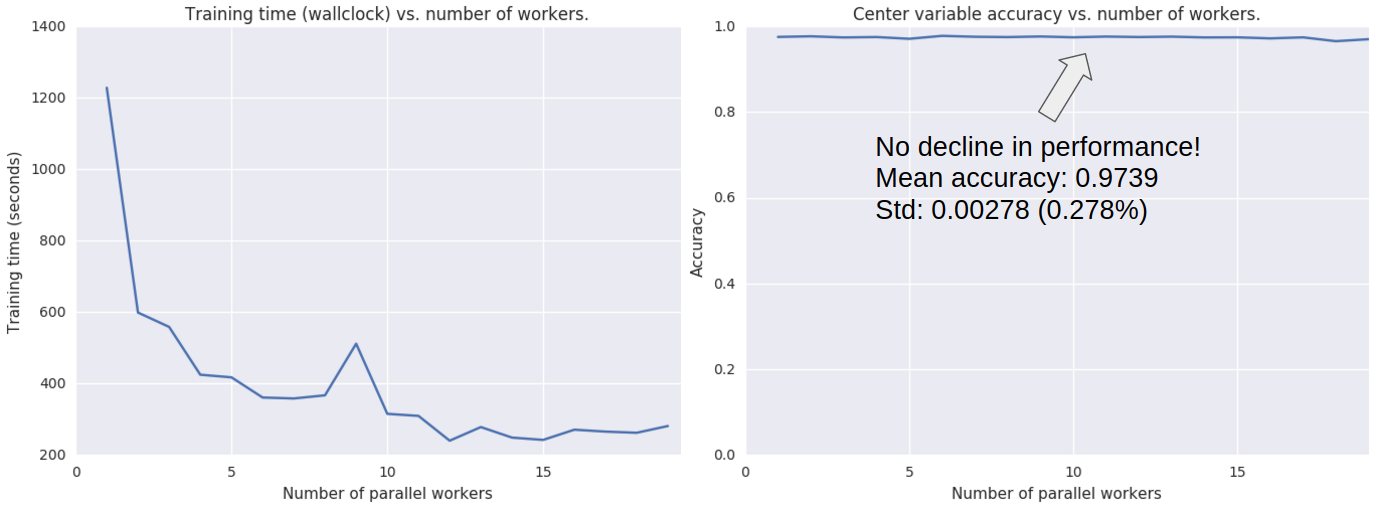
Figure 13: If we would assume no communication constraints, then how would we solve the problem DOWNPOUR has? Averaging the gradients will work, but it is not very desireable since the gradient will act as if they were a sequential optimization algorithm. So what if we would normalize with respect to the communication window? Since this really is the parameter which induces parameter staleness, as can be observed from Figure 12 (declining model performance). An interesting observation we can make here is the absence of any decline in model performance (compared to DOWNPOUR and EASGD). We think this is because one of the following reasons; for one, we keep the variance of the workers small (limited exploration), and normalize the accumulated gradient on the workers with the communication window (which is a prime factor in implicit momentum).

Influence of the communication window on accuracy and training time

In the following set of experiments we will investigate the influence of the communication window on accuracy and training time. The communication window is a hyperparameter which defines the frequency of communication with the parameter server. A communication window of 35 means that a worker will accumulate 35 mini-batch updates, and finally synchronizes with the parameter server. In the experiments, all optimization schemes use identical hyperparameters, where the only variable between tests is the communication window. As before, we will use MNIST as a dataset, a mini-batch of size 4, and Adam as the worker optimizer.

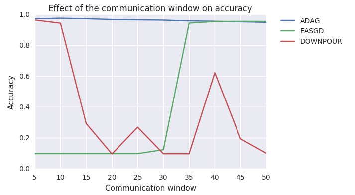
Influence of communication window on accuracy

Figure 14: As expected, DOWNPOUR is not able to handle large communication windows. EASGD on the other hand is not able to handle small communication windows! As stated above, this is because the elastic force (due to the number of workers) is stronger then the exploration of the parameter space. Thus, causing EASGD to not converge. ADAGA on the other hand is able to handle the varying communication window, however, a slight decline in model performance is observed. This is expected due to the increase in exploration of the parameter space by the workers.

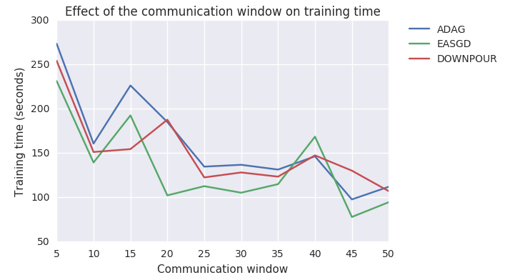
Influence of communication window on training time

Figure 15: Again, the training time of all optimization schemes decrease significantly when the communication window is increased. However, we think we can further decrease the training time by allocated a thread in every worker which sole responsibility is to send the parameters to the parameter server. However, this is an idea that has yet to be explored. To conclude, we suggest to make a trade-off between training time and accuracy, in the case of ADAG, we recommend a communication window of 10-15, since this hyperparametrization achieves similar model performance. However, when applying this to a different dataset. We recommend that you test these settings for yourself, since they can differ.

Summary

In this work we gave the reader an introduction to the problem of distributed deep learning, and some of the aspects which one needs to consider when applying it, such as, for example, implicit momentum. We also suggested some techniques which are able to significantly improve existing distributed optimization schemes. Furthermore, we introduced our framework, dist-keras, and applied different distributed optimization schemes to the MNIST dataset. Finally, we also provided several production-ready examples and notebooks.

Acknowledgements

This work was done as part of my Technical Student contract at CERN IT. I would like to thank Zbigniew Baranowski and Luca Canali of the IT-DB group, Volodimir Begy of the University of Vienna, and to Jean-Roch Vlimant, Maurizio Pierini, and Federico Presutti (CalTech) of the EP-UCM group for their collaboration on this work.

Distributed Deep Learning - Part 1 - An Introduction

Introduction

Model parallelism

Data parallelism

Approaches

Synchronous Data Parallel Methods

Model Averaging

EASGD

Asynchronous Data Parallel Methods

Asynchronous EASGD

DOWNPOUR

ADAG

Experiments

DOWNPOUR

Asynchronous EASGD

ADAG

Influence of the communication window on accuracy and training time

Summary

Acknowledgements

References

- Mitliagkas, I., Zhang, C., Hadjis, S., & Ré, C. (2016). Asynchrony begets Momentum, with an Application to Deep Learning. arXiv preprint arXiv:1605.09774.
- Dean, J., Corrado, G., Monga, R., Chen, K., Devin, M., Mao, M., ... & Ng, A. Y. (2012). Large scale distributed deep networks. In Advances in neural information processing systems (pp. 1223-1231).
- Zhang, S., Choromanska, A. E., & LeCun, Y. (2015). Deep learning with elastic averaging SGD. In Advances in Neural Information Processing Systems (pp. 685-693).
- The MNIST database, of handwritten digits.